Radial interpolation around a point
Time to dust off the old trigonometry magicks
2023-12-07
A radially interpolated circle around a point, all done in fresh, ethically raised, free-range R.
Towards the end of this summer, I was working on a project that involved tracking seabirds, specifically marbled murrelets, flying over radar stations. As a murrelet flew over a particular station, it would be picked up by the radar and the field technician noted the time of day, flight speed, and heading, in degrees, of the little radar blip crossing the screen. We needed a way to estimate the area of land the birds were accessing. Part of the solution: let the birds tell us where they go!
Theoretically, this wasn’t that complicated - I just wanted to create a conical gradient around my headings. The idea here is to create a circle of probability around the heading, where if the raster value is 0, the bird is highly likely to go there, but if the value is 1, the bird is highly unlikely to go there. This is laughably easy to do with built-in functions in a lot of the web design world (such as conic-gradient() in CSS), but I struggled to find an R solution to use with my GIS data. So, I extracted the birds' headings from my data, then spent many, many hours dusting out the trigonometry cobwebs in my brain to come up with this solution.
Without further ado:
# Turn off annoying scientific notation
options(scipen=999)

# Create a dummy data point, and pretend it's somewhere in BC
pt <- sf::st_point(c(-126, 53)) |>
  sf::st_sfc(crs = 4326) |>
  sf::st_transform(crs = 3005)

# Our x, y is no longer in lat/long:
pt
> Geometry set for 1 feature
> Geometry type: POINT
> Dimension:     XY
> Bounding box:  xmin: 1000000 ymin: 888025.7 xmax: 1000000 ymax: 888025.7
> Projected CRS: NAD83 / BC Albers
> POINT (1000000 888025.7)
Let’s set up some other parameters of interest. For this example, I’m interested in interpolating my raster to a distance 30 km away from my data point for a bird flying at a 45° heading. Keep in mind EPSG 3005 is projected in meters - so 30 km becomes 30,000 m. Because I’m working with raster data, I also need to set the resolution of my pixels. Getting it down to a 1/2 km x 1/2 km square is good enough for me, so I set the resolution to be 500 meters.
Next, I also set three variables that aren’t biologically/geographically of interest, but more “quality of life” type variables to make my code easier to bundle into a function down the line: mask, invert, and maxvalue.
# Biological/spatial variables of interest
radius <- 30000
heading <- 45
res <- 500

# Miscellaneous variables that will come into play later
mask <- TRUE      # Do I want to mask my interpolation into a circle shape, or keep it as a square shape? TRUE/FALSE
invert <- FALSE   # Do I want to invert my raster values (so it runs from 1 to 0 instead of 0 to 1)? TRUE/FALSE
maxvalue <- 1     # What do I want the maximum value of my raster to be? Here I set it to 1.
Now comes the hard part: the trigonometry!
# Convert heading degrees to radians
# This is sloppy trig, but it works, so......
# 1) Multiply heading by -1 to ensure radians go clockwise (radians are measured counter-clockwise, by default)
# 2) Multiply by pi/180 to convert to radians
# 3) Subtract from 180° to rotate the angle (radians by default are measured from the x-axis,
# i.e. "east", rather than "north" on a compass-rose)
heading <- (180-heading) * (-pi/180)
# Check out our heading value now - it's in radians!
heading
> [1] -2.356194
# Buffer our point by our radius (30km)
p_buff <- sf::st_buffer(pt, radius)
p_buff <- terra::vect(p_buff)
## Rasterize it to 500m resolution
cone <- terra::rast(p_buff, resolution = res)
# Extract our (x,y) coordinate values
xy <- suppressWarnings(terra::crds(cone))
# To visualize:
# It's just a grid, with points spaced out every 500 m
# (our resolution specified in the function args above)
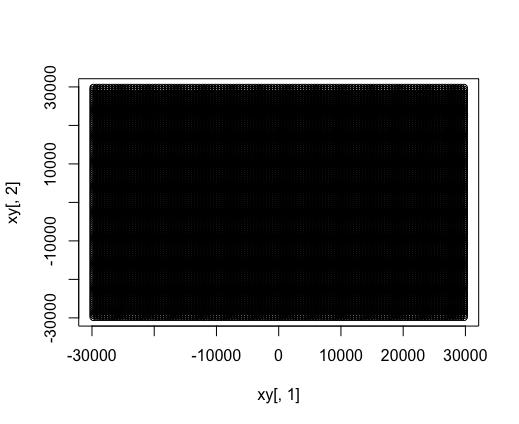
plot(xy[,1], xy[,2])
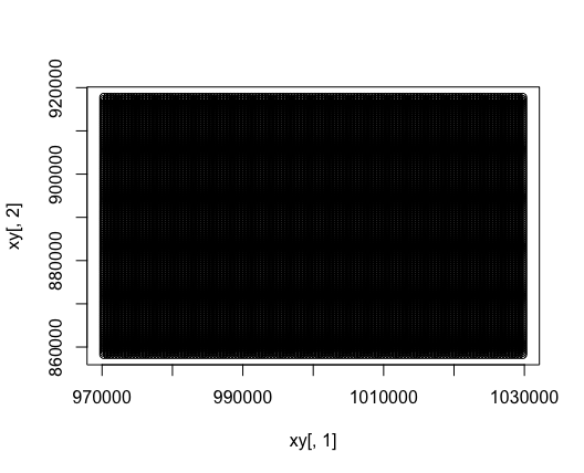
Gridded (X,Y) data at a 500m resolution. (X,Y) values here represent easting, northing coordinates in the EPSG 3005 projection.
# Adjust our grid to show distance from origin, rather
# than absolute coordinates
xy[,1] <- xy[,1] - sf::st_coordinates(pt)[1] # x col becomes x distance from origin
xy[,2] <- xy[,2] - sf::st_coordinates(pt)[2] # y col becomes y distance from origin

# To visualize:
# The same 500 m resolution grid, but x & y now represent
# distance from the origin rather than absolute coordinates.
# The origin now becomes (0,0).
plot(xy[,1], xy[,2])
Gridded (X,Y) data at a 500m resolution, with (X,Y) values now representing distance from the origin in meters.
Next comes the radial interpolation. We need to fill in these (X,Y) values in the raster grid with values running from 0 to maxvalue (which we set to = 1, above), radiating out from the 45° heading.
# Take the arctan of each point
# Arctan: given a vector (x, y), returns angle `v`
# from the x-axis
# CAVEAT: for some reason the `atan2()` function
# takes the y argument first!! See `?base::atan2()` for details.
# `v` is expressed from `-π ≤ θ ≤ π`, i.e. radians
v <- atan2(xy[,2], xy[,1])

# To visualize:
library(ggplot2)
ggplot() + geom_point(aes(x = xy[,1], y = xy[,2], color = v))
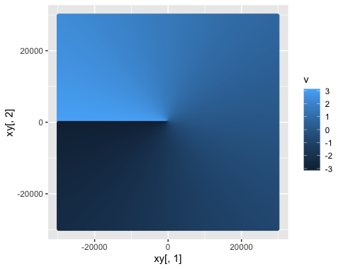
Gridded (X,Y) data at a 500m resolution, with (X,Y) values representing distance from the origin in meters, colored by v, the arctan value (aka, angle, in radians, from the zero axis!) at each coordinate. Notice the color scale runs from -π to +π!
It looks a little funky with the line running down the left - but that is because radians start from the +x-axis (y = 0, x > 0), or 90°/East on a compass rose. So, given an angle v of:
- 0 = +x-axis = 90°/East
- π/2 = +y-axis = 0°/North
- π = -x-axis = 270°/West
- -π/2 = -y-axis = 180°/South
- -π = -x-axis = 270°/West
So every point on our x,y grid now has a v angle from the origin associated with it, representing the angle from the x-axis, or 90° due East.
Now we need to re-scale everything so that it actually runs from 0 (our desired heading) to 1 (opposite our desired heading). At the moment our scale runs from -π ≤ v ≤ π, as measured as the angle from 90° due east. Not helpful. Instead, we want all our cell values to show us the angle from heading, with 1 = heading and 0 = opposite heading.
If we continue dusting off our old trig knowledge… the sine of an angle = the opposite side/hypotenuse. Functionally what this means is that if our line lies flat along the x axis, our angle is zero, and therefore the sine of our angle = 0.
If we add our heading angle, we will ‘rotate’ the axis that the sine measurement is taken from, so we can incorporate heading of interest in our cone.
# To visualize:
# Without rotation - sine measures the angle from x-axis:
ggplot() + geom_point(aes(x = xy[,1], y = xy[,2], color = sin(v)))

# With rotation - sine measures the angle from our heading of interest, `heading`:
ggplot() + geom_point(aes(x = xy[,1], y = xy[,2], color = sin(v + heading)))
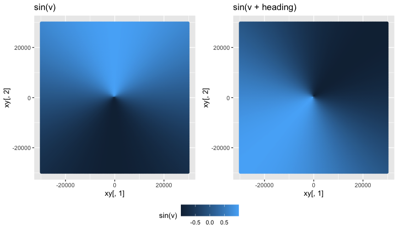
Left: sine of our angles, v, as measured from the x-axis (90° due East per compass rose). Right: sine of our angles v PLUS our heading (which is in radians now). Note the difference in the angle that our color gradient changes.
From here it’s simple arithmetic to re-scale our numbers from 0-1 instead of 1-1.
# Re-scale our numbers from 0-1 instead of -1-1
cone[] <- (1 + sin(v + heading))/2
# If we want to invert it, such that 0 = heading and 1 = opposite heading,
# that's also pretty simple (recall we set `invert <- TRUE` above):
if (invert) cone[] <- (cone - 1) * -1
# If we want our numbers to run from 0-something else, it's a simple
# multiplication (recall we set `maxvalue <- 1` above):
cone[] <- cone * maxvalue
# Finally, we mask it with our circle buffer to produce a circle output
# (recall we set `mask <- TRUE` above):
if (mask) cone <- terra::mask(cone, p_buff)
# Easier to switch to terra at this point to quickly visualize raster data
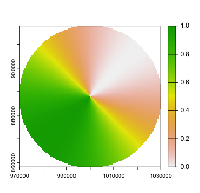
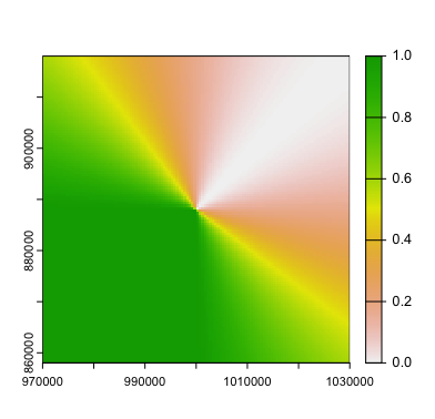
terra::plot(cone)
Hey! It’s the picture from the top of the blog post!
ADVANCED CONE MANIPULATION
That’s right, you’re ready for this. It’s what you’ve always dreamed of achieving, right?
Let’s say we want to interpolate across a narrower or wider cone angle that we can specify. Let’s call that angle theta. Let’s also say we want the area of our cone where (x,y) = 1 to be fully 1/4 or our circle.
# Let's interpolate across a wider cone angle. I want fully 1/4 of my circle to = 1.
theta <- 90 # 1/4 of a circle is 90°
theta <- theta * (pi/180) # Multiply by pi/180 to convert to radians
# Instead of taking the sine of v and immediately normalizing
# to 0-to-1, we just take the sine (+ heading to rotate).
v2 <- sin(v + heading)
# Except now anything > cos(theta/2) = 1, and
# anything <= cos(theta/2) interpolated to 0-1
# To visualize:
cone[] <- v2
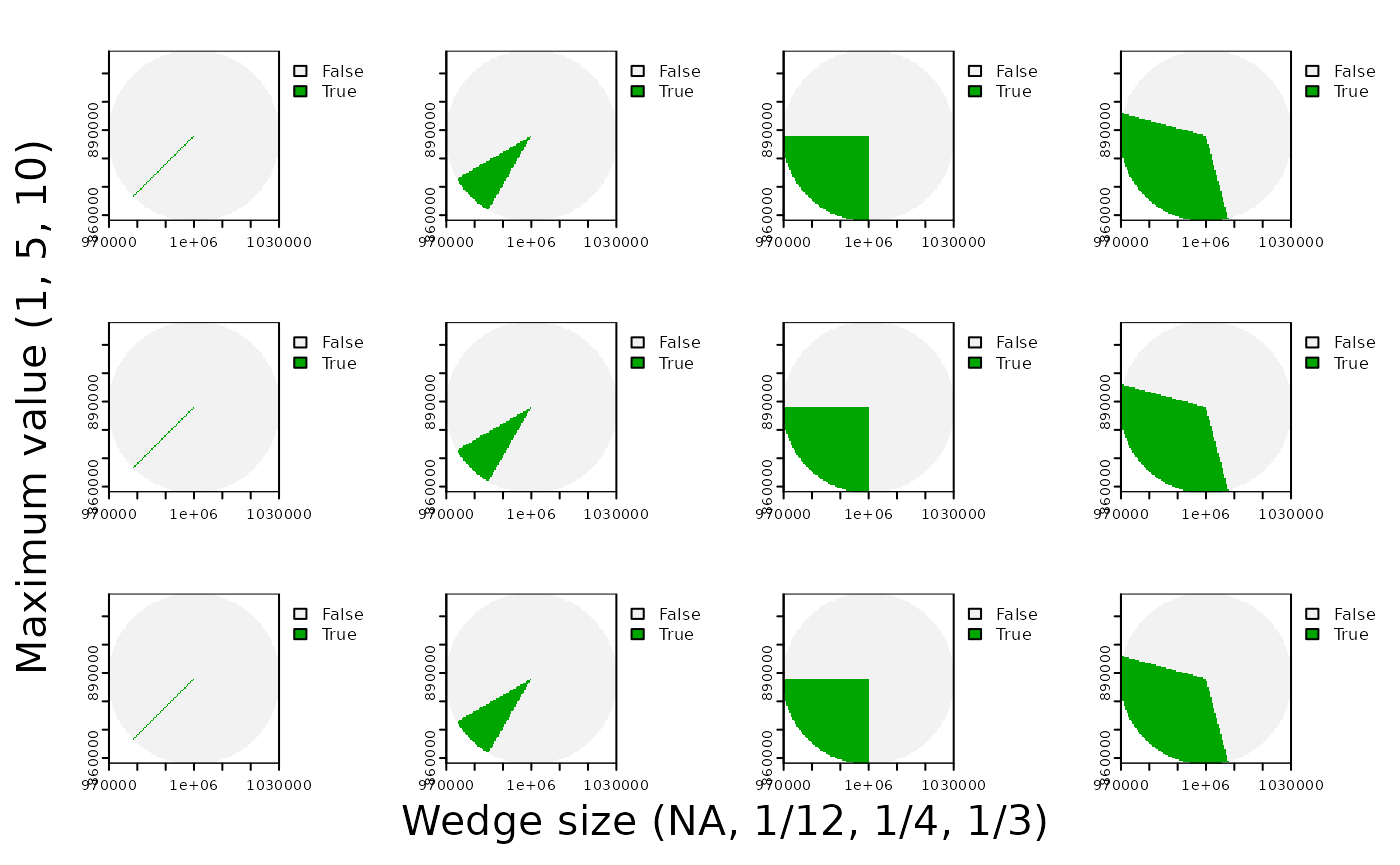
terra::plot(cone > cos(theta/2))
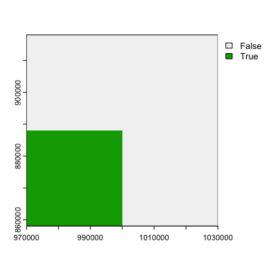
1/4 of our grid is now cordoned off to be a set value of 1. We will now radially interpolate in the intervening grey space.
#Now we re-scale so that the 1 on our 0-1 scale
# corresponds to cos(theta/2)
v3 <- (v2 - min(v2)) / (cos(theta/2) - min(v2))
v3[v3 > 1] <- 1

cone[] <- v3
terra::plot(cone)
Interpolated values from our 45° heading, but with only 3/4 of the circle interpolated. The other 1/4 of the circle we manually set to be 1 (dark green).
VOILA.
BRING EVERYTHING TOGETHER INTO ONE NEAT FUNCTION
Typing and re-running all that would get tiring, no? Let’s bundle it together into a function.
radar_cone <- function(pt, radius, heading,
                       theta, res, mask,
                       invert, maxvalue) {
  # Data health checks
  # Check that pt is a sf point object
  stopifnot("`pt` must be a sf POINT feature." = inherits(pt, "sfc_POINT") == TRUE)
  # Check that radius > 0
  stopifnot("`radius` must have a positive value." = radius > 0)
  # Check that theta >= 0
  stopifnot("`theta` must have a positive value." = theta >= 0)
  # Check that res > 0
  stopifnot("`res` must have a positive value." = res > 0)

  # Convert degrees to radians
  # This is sloppy trig, but it works, so......
  # 1) Multiply heading by -1 to ensure radians go clockwise (radians are measured counter-clockwise, by default)
  # 2) Multiply by pi/180 to convert to radians
  # 3) Subtract from 180° to rotate the angle (radians by default are measured from the x-axis,
  #     i.e. "east", rather than "north" on a compass-rose)
  heading <- (180-heading) * (-pi/180)
  p_buff <- sf::st_buffer(pt, radius)
  p_buff <- terra::vect(p_buff)

  ## Rasterize it to 500m resolution
  cone <- terra::rast(p_buff, resolution = res)
  xy <- suppressWarnings(terra::crds(cone))

  xy[,1] <- xy[,1] - sf::st_coordinates(pt)[1] # x col becomes x distance from origin
  xy[,2] <- xy[,2] - sf::st_coordinates(pt)[2] # y col becomes y distance from origin

  # Take the arctan of each point
  # Arctan: given a vector (x, y), returns angle `v`
  # from the x-axis in radians such that `-π ≤ θ ≤ π`
  v <- atan2(xy[,2], xy[,1])

  # Adjust values to fall along our heading of interest
  v2 <- sin(v + heading)

  # Re-scale values from 0-1 instead of -1-1
  # If theta = 0 (default), the output produces a smooth
  # linear interpolation from 0-1 around the whole circle.
  # If theta > 0, a wedge with an angle of theta degrees
  # will be set to 1.
  theta <- theta * (pi/180) # Multiply by pi/180 to convert to radians
  v2 <- (v2 - min(v2)) / (cos(theta/2) - min(v2))
  v2[v2 > 1] <- 1

  # Fill in cone values
  cone[] <- v2

  # Invert such that 0 = heading and 1 = opposite heading
  if (invert) cone[] <- (cone - 1) * -1

  # Adjust scale that is output
  cone[] <- cone * maxvalue

  # Mask to circular output
  if (mask) cone <- terra::mask(cone, p_buff)

  return(cone)
}


terra::plot(radar_cone(pt = pt,
                       radius = 30000,
                       heading = 45,
                       theta = 0,
                       res = 500,
                       mask = TRUE,
                       invert = FALSE,
                       maxvalue = 1))
Wait a second. That’s the plot from the top of the blog post for a third time, isn’t it?!
terra::plot(radar_cone(pt = pt,
                       radius = 45000,
                       heading = 106,
                       theta = 30,
                       res = 500,
                       mask = FALSE,
                       invert = FALSE,
                       maxvalue = 15))
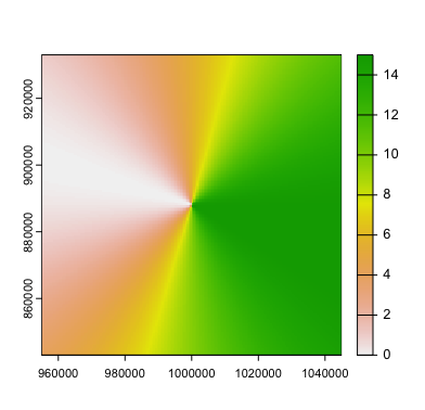
Much better.
Miscellanea
Big thanks to Spacedman on GIS StackExchange for helping me get this code off the ground.
The function here was developed with support from Environment & Climate Change Canada for the {MAMU} package, a suite of R tools to analyze marbled murrelet data in British Columbia. A small vignette of the function is online here.